

How to look like a pro when using Microsoft Excel
- Emil Lazar

- Feb 17, 2021
- 8 min read
Microsoft Excel is a helpful and powerful piece of software for data analysis and documentation. It is a spreadsheet program, which contains a number of columns and rows, where each intersection of a column and a row is called a cell.
If you're just starting out and are looking to impress a colleague, your boss or a client with your — real or apparent — Excel skills, we're going to show you some easy hacks you can adopt from the toolset of Excel professionals. Although professional Business Analysts regularly use advanced formulas, pivots, macros/VBA, Microsoft SQL Server, Power BI integration and perhaps many other analysis tools and add-ons, we'll focus on things you can easily learn and implement to appear like a pro without actually having to learn all the hard stuff. The world of Microsoft Excel is huge and no single article can contain everything it has to offer.
The key to getting to be a pro is "fake it 'till you make it". Get comfortable with Excel, persist, be curious, and you'll see yourself become a professional.
Table of contents
Keyboard shortcuts
Pros will avoid using the mouse — or will use both mouse and keyboard at the same time— because using just the mouse will slow them down. The keyboard can help you do so much more in so little time. Start by adding basic keyboard shortcuts to your Excel routine, use them until they become natural, then learn some more. The amount of possible keyboard shortcuts can be overwhelming, so try incorporating only a few at a time. We recommend mastering the below shortcuts first, then graduating to more advanced ones.
1. Edit shortcuts:
Ctrl (or ⌘ on Mac) + C - Copy
Ctrl (or ⌘ on Mac) + V - Paste
Ctrl (or ⌘ on Mac) + X - Cut
Ctrl (or ⌘ on Mac) + Z - Undo
Ctrl (or ⌘ on Mac) + Y - Redo
Ctrl (or ⌘ on Mac) + S - Save
2. File navigation
Ctrl (or ⌘ on Mac) + ↑, Ctrl/⌘ + ↓, Ctrl/⌘ + ←, Ctrl/⌘ + →
These are your navigation keyboard shortcuts. They can go to the very last column or line of data in your file (very useful if you have a lot of columns/lines).
3. Cell navigation
When you're new to Excel, sometimes the cells and their content may behave differently from what you may have expected them to. This depends on the combination of keys used.
When you're in "viewing" mode and are just browsing, the arrow keys (↑, ↓, ←, →), will move around one cell in each direction.
However, when you're in "data entry" mode and you want to move to a certain direction after you're done, you'll need to use the following key combinations:
Enter (or ⏎ on Mac): advance to the cell below the current selected one
Shift + Enter (or ⏎ on Mac): advance to the cell above the current selected one
Tab: advance to the cell to the right of the current selected one
Shift + Tab: advance to the cell to the left of the current selected one
F2: edit cell contents or formula (mouse equivalent is double-click).
This can help you pinpoint a precise change inside the cell. Not pressing F2 beforehand replaces all content with the newly typed text. The video to the right shows what happens in both cases.
4. Selection
Ctrl (or ⌘ on Mac) + A: Selects all cells in a worksheet. If the worksheet contains data, and the active cell is above or to the right of the data, pressing Ctrl/⌘ + A will select the current region. Pressing Ctrl/⌘ + A a second time will select the entire worksheet.
Ctrl (or ⌃ on Mac) + Shift + 8: Selects all cells in the active range.
What's the difference between the two? The video above shows selecting the active range first then the entire worksheet.
If you want to select a large range of cells, instead of clicking with the mouse, holding and dragging all the way to select this range, try clicking on the top right cell first and going to the bottom right one and selecting it after pressing Shift. Much faster!
Basic calculations
If you want a cell to display a calculated result, select the cell, press "=" then use cells and. operators (+, -, *, /), as desired. In this case, we'll use the mouse to move around and the keyboard to select the operators. No time wasted!
Remember, pros don't use Calculator, they use Excel.
Quick operations
When selecting a range of cells, Excel can show you some quick calculations in the bottom bar:

You can customize what is displayed by right clicking the quick calculation area :
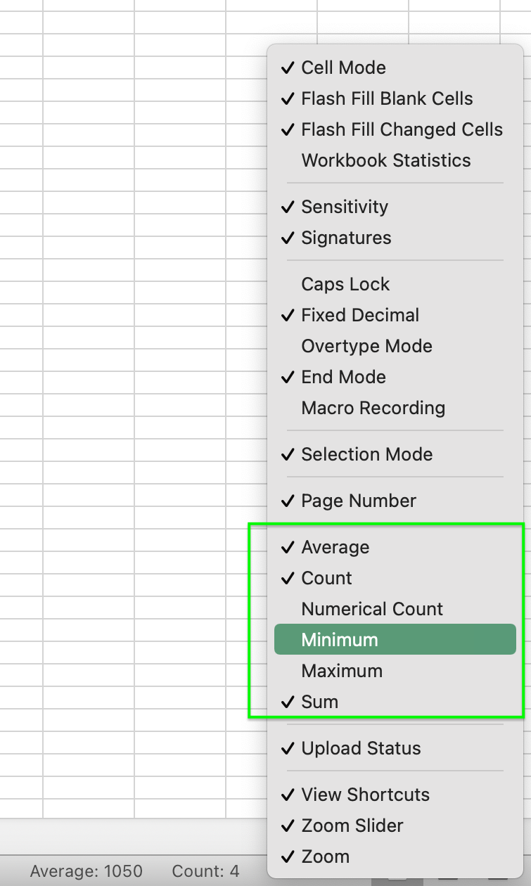
The difference between Count and Numerical count is that Count is displaying the number of cells with data and Numerical count is displaying the number of cells which contain only numbers.
AutoSum
AutoSum is a handy feature of Excel that contextually calculates the sum relative to the selected cell. This can be activated by pressing Alt + = in Windows or shift + ⌘ + T on Mac. On Windows, you have the option of fine-tuning the selection before hitting Enter to execute the formula. You will most likely use this at a bottom of a column.
Quickly copy a cell
Ctrl (or ⌘ on Mac) + D: copy contents from the above cell to the selected one
Ctrl (or ⌘ on Mac) + R: copy contents from the left cell to the selected one
Quickly copy a formula across a column
You can use the above mentioned Ctrl (or ⌘ on Mac) + D, drag or double-click on the lower-right corner of the cell, depending on how much of the formula you want copied.
VLOOKUP
The VLOOKUP formula is a milestone whose mastery can attest you're no longer an Excel beginner.
VLOOKUP (and its much less used cousin HLOOKUP) are formulas that can bring order to the report you're trying to pull together. If you find yourself in a situation where you have some data, but it's not assembled in an useful way for your report, VLOOKUP can help.
In the below example, we have four regions (North, South, East and West) and an Area Sales Manager for each of these regions. In the highlighted area, we'll need to fill in the respective Area Sales Manager. While for smaller scale cases (such as this one) we can manually input the right answer just by looking at the right side of the file, as tables grow larger, it will make manual solutions less and less feasible.

This is a one-to-one association. VLOOKUP won't work in one-to-many or many-to-many relationships as it may display unreliable data.
We'll start by selecting cell E3 and entering the VLOOKUP formula. We'll need the following:
what to tell VLOOKUP to look for
where to look it up
which column to look for (or which line in HLOOKUP)
whether we want an exact or an approximate value returned
So, for the first line, line #3, the answer to these is the following:
what to tell VLOOKUP to look for the value of cell B3 (Region)
where to look it up in the area between cell G3 and H6 (Region and Area Sales Manager)
which column to look for we'll need the second column (Area Sales Manager)
whether we want an exact or an approximate value returned as a best practice, we want an exact value (for North, this should be Francisco)
There are a number of precautions to take in order to have a correct result displayed by VLOOKUP and as a best practice, instead of selecting area between G3 and H6, we'll tell Excel to select the entirety of columns G and H — provided we don't have any other data which can interfere with our results lower on these columns).
Let's see how we translate this into Excel language.
what to look for B3
where to look it up G:H
which column to look for 2
whether we want an exact or an approximate value returned FALSE (the question is "approximate?" and we reply with FALSE — we don't want an approximate)
Putting it all together, we will type the following into cell E3:
=VLOOKUP(B3,G:H,2,FALSE)
Here's how it looks like in action:
Finally, we'll do a sample check to verify that the formula is working and we should be all set.
If we're done with the formula, it's a good idea to copy the VLOOKUP calculated area and paste as values, in order not to be dependent on the referenced source, which may move or alter in ways we don't want it to.
If you're new to VLOOKUP, it might take you a few tries to get this right. Keep practicing and don't give up. This is an essential formula that will save you a considerable amount of time and will serve you well.
Freeze Panes
Freeze Panes is great when you have a large number of lines and/or columns and you want to keep that header or first column.
To enable the view, select the a cell. Anything to its left and top will be fixed while all the other cells will be movable.
The go to the View tab in the Ribbon and select Freeze Panes. Upon selecting it, with each successive click, it will toggle between Unfreeze Panes and back to Freeze panes. The reason for this is that Freeze Panes cannot be undone with Ctrl (⌘) + Z.
Conditional formatting
Most people are visual, meaning that they can easily interpret data if it has colors, graphs or cues that help understand a table of values. This is where Conditional Formatting comes in.
Relative conditional formatting
If you'd like to see how well Area Sales Managers are performing relative to each other, you will use this method. Select the area which contains the data you want analysed, go to the Ribbon, selecting the Home tab and then Conditional Formatting. For our case, we'll select a color scale:
Red = below average
Yellow = average
Green = above average
Depending on your audience, you may want to select a scale which is high contrast or colorblind friendly.
Here's how it looks like in Excel:
Easy, right? Now you can spot your top performers in a quick glance. This is called relative because the Area Sales Managers are not being measured against a benchmark or an imposed target, but just amongst each other.
Absolute conditional formatting
If you want to make sure that your Area Sales Managers are challenged and are actually doing a world-class job, you might want to introduce an objective benchmark or a target. Let's say this is 4000. We'll go to the Ribbon, select the Home tab and then Conditional Formatting (just as before), but we'll go to Manage rules instead. Here, we'll create a new rule in a 3-Color Scale format, pick our Midpoint as 4000 and select our colors according to our theme. We'll keep the existing Red Yellow Green one.
Sounds complicated? Take a look at how easy this actually is in Excel:
Well what do you know, our sales organization is doing fabulous! Except for Malika — maybe. Let's not be so quick to judge her, we still don't know the full picture, maybe the East region market is tough, has reached maturity, or facing other challenges. Maybe Malika's new on the job and just needs some training. Or, maybe the other three are exceptional Area Sales Managers and Malika is just great. Whatever it is, we need more data before we can jump to conclusions.
As mentioned at the beginning of the article, Microsoft Excel is a whole universe. While we can't possibly cover all the tips, tricks and features of this software, mastering the easy basics covered in this article will provide you with powerful ways to tame data — and impress along the way.


Comments